Tesla's Colorado Springs Receivers

(A Short Introduction)

"While experimenting in Colorado...I had perfected a wireless receiver of extraordinary sensitiveness, far beyond anything known."

Nikola Tesla (Albany Telegram, February 25, 1923)

§1 Introduction*

A significant segment of Nikola Tesla's 1899 Colorado Springs research effort encompassed the detection and monitoring of VLF radio waves emitted from atmospheric electrical storms. (Twenty-nine years later, Karl Jansky was conducting much the same research, at short-wave, when he observed thunderstorms and discovered radio noise emanating from the galactic plane.) Indeed, this branch of radio science may be traced directly to Tesla. Tesla also reported detecting a peculiar extra-terrestrial signal, which he subsequently concluded was from the planet Mars. How did the1899 receivers of Tesla's work?

Using Tesla's patent applications, correspondence, and Colorado Springs laboratory notes¹ (abbreviated as CSN), about 15 years ago we conducted a study of his novel coherer techniques and reconstructed models of his receiving apparatus. The results were surprising to us, for they revealed an unanticipated level of sophistication not initially apparent in the simple circuit diagrams. His 1899 coherer operation was nothing like the coherer circuits of Branly, Lodge, or Bose. Not only did Tesla's detector circuits include high Q tuned resonators, but also oscillator injected negative resistance [similar to the peak (or "boost") operation of the shunt type Q-multipliers of the 1950s, which raised the effective Q and increased the resonant rise of voltage]. This has the same effect as making the detector stage regenerative. A detailed technical discussion of Tesla's 1899 receivers was published in 1994,² and an analysis of the "radio telescope" system parameters associated with his Colorado Springs observatory was presented in 1996.³ As with Armstrong's super-regenerative receiver, which was patented in 1922, Tesla's sensitive detectors require only a few components and are deceptively simple.

§2 Tesla's Receiver Drawings

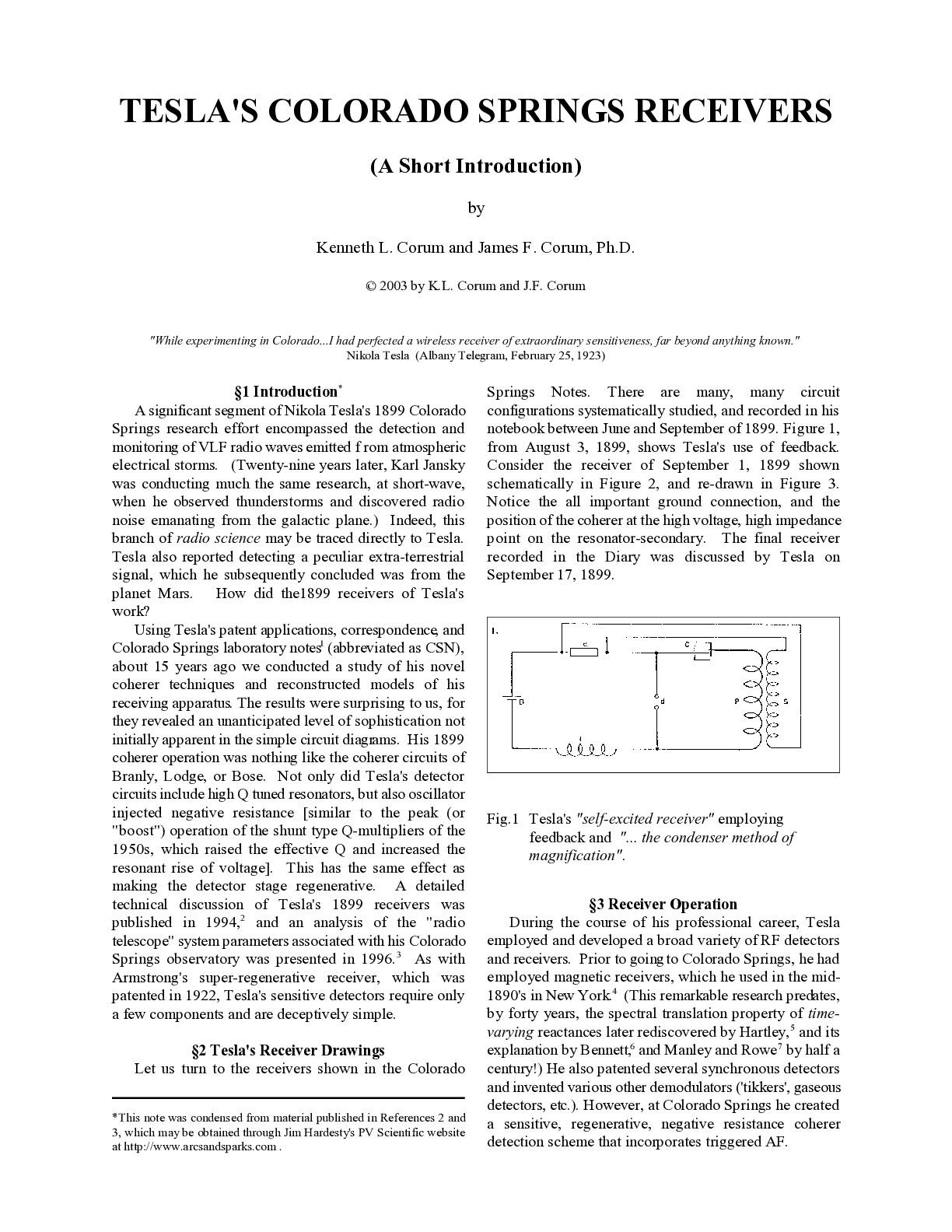
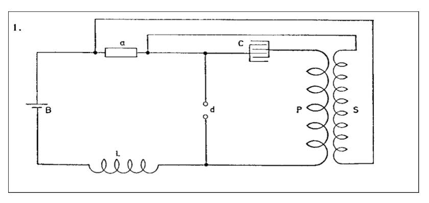
Let us turn to the receivers shown in the Colorado Springs Notes. There are many, many circuit configurations systematically studied, and recorded in his notebook between June and September of 1899. Figure 1, from August 3, 1899, shows Tesla's use of feedback. Consider the receiver of September 1, 1899 shown schematically in Figure 2, and re-drawn in Figure 3. Notice the all important ground connection, and the position of the coherer at the high voltage, high impedance point on the resonator-secondary. The final receiver recorded in the Diary was discussed by Tesla on September 17, 1899.

 §3 Receiver Operation

During the course of his professional career, Tesla employed and developed a broad variety of RF detectors and receivers. Prior to going to Colorado Springs, he had employed magnetic receivers, which he used in the mid-1890's in New York.⁴ (This remarkable research predates, by forty years, the spectral translation property of time-varying reactances later rediscovered by Hartley,⁵ and its explanation by Bennett⁶, and Manley and Rowe⁷ by half a century!) He also patented several synchronous detectors and invented various other demodulators ('tikkers', gaseous detectors, etc.). However, at Colorado Springs he created a sensitive, regenerative, negative resistance coherer detection scheme that incorporates triggered AF.

§3.1 Circuit Components

Most of the circuit elements in the schematic diagrams are self-evident. However, let us call attention to some of the (now) unconventional symbols and components that Tesla employed in his drawings.

(a) The element marked "R" was called the receiver, which was merely a relay, Morse telegraph sounder, or telephone receiver - a high impedance earphone (which Tesla sometimes referred to as a "telephone"). The component, R, was simply the radio receiver's electromechanical output transducer (and not what we would call a "receiver" today).

(b) The two nodes marked by small circles ("d") was an electromechanical switch that was commonly called a break or circuit interrupter. Tesla referred to breaks as "circuit controllers", and h e took out many patents on this technology during the 1890s. The break permitted the control of repetitive switching transients: capacitor charging and discharges. With breaks, one could control the pulse repetition frequency (in pulses per second) and also the pulse duration.

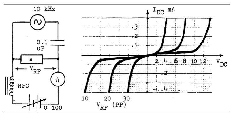
(c) The construction and characterization of the coherer(element "a") is discussed in great detail in Tesla's notes and in several of his patents. (See the footnote at the close of section 3.4 below.) Historically, the early application of the coherer was for an RF "detector", not in the sense of how we use "demodulators" today, but rather for determining whether RF was present or not present. As a result of experimental measurement, we noted that as the RF voltage across the device was increased, the DC resistance decreased, from 1 megohm down to 50 ohms.** (The coherer's DC resistance vs. RF signal voltage is discussed in Ref. 2.) The resistance then remained almost constant until the voltage was raised to an avalanche point, where the device became a short. With the RF removed, if the device was tapped then its resistance resumed the 1 megohm value. The RF sensitivity of the detector is highest for device ingredients with the steepest slopes for DC resistance vs. RF bias, e.g. tiny particles of silver. The measured family of coherer characteristic curves is shown in Figure 4.

The facts that the coherer's characteristic curves are nonlinear and nonuniformly spaced, and that the device decreases its resistance with increasing amounts of RF bias, makes it a unique component. However, in Tesla's mode of operation the coherer holds one more surprise.

§3.2 Regenerative Process

Bearing the conventional electrical characteristics in mind, one might want to apply a small amount of locally generated RF and a DC bias to push the coherer device toward the knee in the resistance transition, making it more sensitive to low voltage RF signals. (At the knee of the characteristic curve, the forward and reverse resistances are substantially different.) Remarkably, this idea of employing locally generated RF in conjunction with a coherer shows up again 18 years later in the discussion following Edwin Armstrong's pioneering publication on regenerative detectors. (Regeneration, is the process of supplying energy to a circuit to reinforce the oscillations existing in it.) A workable technique for regeneration (positive feedback) by self-heterodyning is commonly traced to Armstrong, and in 1917 Armstrong published a masterful engineering study of the phenomenon.⁸ He discovered that appropriately phased RF feedback⁹ of a received signal, coupled from a single-stage plate circuit back to the grid circuit, would make an extremely weak received carrier signal grow in amplitude, virtually to the point of overload distortion. [In a conventional regenerative detector, the plate circuit current has two spectral components, one is the demodulated baseband signal and the other is an amplified RF signal. The high frequency component of the plate current is coupled back through a tickler coil to the grid and serves for RF amplification (regeneration), and the baseband component of the amplified plate current provides the output detected signal in this remarkable receiver circuit.¹⁰] At that time, voltage gains of 35 dB could be attained from a vacuum tube operating as a grid biased Class A amplifier (which was invented and patented by Tesla's assistant, Fritz Lowenstein,¹¹ the IRE's first Vice-President when it was formed in 1912). But, Armstrong's approach gave RF gains in excess of 74 dB with the available tubes of that day!

Is a triode, or three element device, required for this process? No. The overall process of regeneration is equivalent to passing a signal through a tuned tank circuit into which a negative resistance has been injected. (RF feedback amplification is the mechanism by which negative resistance arises in the tank circuit in Armstrong's embodiment.) The result is to neutralize the positive (loss) resistance of the tank. Not only does the amplitude of the RF signal grow (the amplification is limited by the tube breaking into self oscillation), but the tank circuit's Q
multiplies as the net loss decreases.^12,13 Similar results can be obtained with any negative resistance component, such as a tunnel diode, which is a two terminal device.

In the discussion correspondence following Armstrong's 1917 regeneration paper, Carl Ort¹⁴ points out that in Austria he and his colleagues obtained gains of 20-fold (26 dB) when using coherers made "very sensitive" by local oscillator RF injection. (This regenerative process is not the superheterodyne principle.¹⁵ Neither is it super-regeneration,^16,17 which provides sensitivity right down to the thermal noise floor.) IRE Vice-President J.V.L. Hogan found that the increase in receiver sensitivity was even obtained when RF injection was employed with a crystal detector.¹⁸ According to Ort's 1917 remarks the reason for the great gain was never understood until Armstrong's landmark regeneration investigation.

"Mr. Armstrong's experiments have shed new light on these phenomena and have indicated that the amplification obtained with a rectifying detector depends on the energy of the local oscillations which are applied to the detector, and that, while the energy received is not magnified at all, the sensitiveness of the detector is increased. This increase is independent of the frequency of oscillation of the local source."¹⁹

This is remarkably similar to Tesla's description 18 years earlier. Tesla's patents teach us that when his coherer is exposed to an injected RF signal, it behaves as a voltage controlled resistor. He recognized that it was not merely a go/no-go indicator of RF (as originally used by Branly and Marconi²⁰), and not a rectifying diode (as in the Lodge and Bose²¹ envelope detector mode of coherer operation).

§3.3 Negative Resistance

It is true that the coherer's family of characteristic curves (a plot of device current vs. applied voltage for various biases) clearly displays nonlinearity (see Fig. 4), especially for small signals biased out near the knee. But, where is the negative resistance that Ort (and Tesla) observed?

A short discussion of two-terminal negative resistance devices is attached as an appendix below. In the case of a tunnel diode, the current rises with junction voltage (positive resistance), then decreases with further rise in junction voltage (negative resistance), and finally rises parabolically with any further increase in junction voltage. On the characteristic curves shown in Figure 4, suppose the initial coherer operating point is at V_DC = 4 volts, V_RF = 30 volts PP, and I_DC = 0.3 mA. Then, with V_DC = 5 volts, suppose V_RF swings through 25 volts, where I_DC has decreased to 0.1 mA. Clearly, the device would exhibit incremental negative resistance, of value R_n = - 5 kΩ. It would appear that the Local Oscillator RF injection is freely shifting the operating point to make negative resistance occur. If this is true, then the resonator Q would increase substantially.

In our opinion, what Tesla had created was a sensitive, voltage controlled variable resistor with an accessible operating region of negative slope. Tesla's discovery (and documentation by means of patent protection) of this fourth mode of coherer operation not only makes possible a realm of sensitive coherer operation, but also creates an entirely new dimension to receiver architecture.

§3.4 Architecture

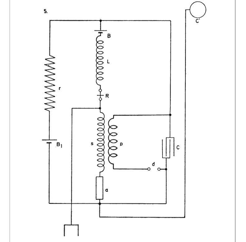
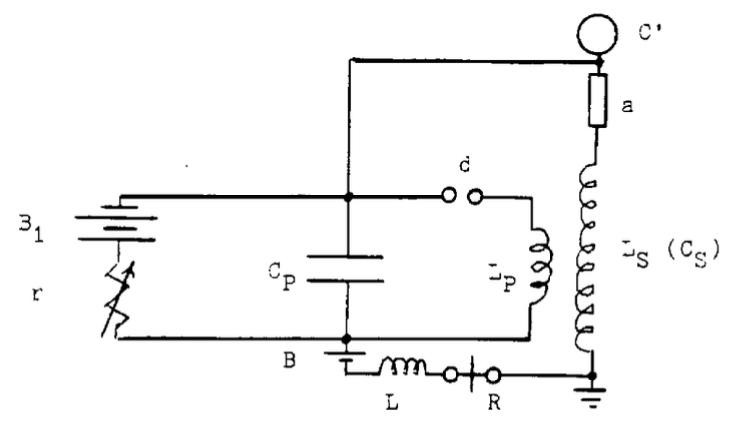
Permit us to emphasize again that the Tesla receiver circuits are deceptively simple! First, notice the architecture of the schematic drawing shown in Figure 3. This is important: there are actually four superimposed circuits:

1. The C_P charging circuit. B₁ charges C_P through resistance r with time constant τ₁ = rC₁. This places a DC voltage on C_P. For reasons which will soon be evident, this will be called the "Sensitivity Control".

2. The L_PC_P damped-wave oscillator including the tightly coupled coils, L_P-L_S, and break d. This is a local RF oscillator, but its output and application are different than the LO for mixer injection taking place in a superheterodyne receiver. Tesla's LO generates double-peaked high voltage RF (on the order of several hundred volts) in a shaped passband to impress upon the coherer device "a". Note the position of "a" at the top of the secondary coil, or resonator stage. The bottom of the secondary coil is grounded.*** When the coherer's resistance is high (- 1MΩ) its presence will not impact the operation of the LO circuit.

3. A baseband detector stage, which operates while the break device (d) is closed. This consists of the coherer "a", the primary inductor LP, the secondary coil L_S (which at baseband behaves as a low impedance resistance - 50S for a DC return path for battery B through the coherer "a"), and the indicator R (a 900 S DC relay, telegraph indicator, or earphone) which is battery driven. The coil L is an RF choke to provide a high impedance to any RF in the baseband AF stage.

4. The antenna-ground circuit, which provides the input RF signal. This circuit consists of the antenna capacitance C', the coherer device "a", the resonator coil LS, and the ground connection, which is most important. The resonator is "tuned" to the desired frequency of reception as shown in Tesla's patents. When there is no RF signal between C' and ground, the coherer resistance is high (- 1MΩ). When RF signals of sufficient strength are present, the coherer resistance drops considerably (ultimately to about 50Ω). The LO injection through the coupled coils establishes the initial operating point on the coherer's characteristic curves.

As mentioned above, the sensitivity of the classical Branly coherer was known to be quite poor, requiring signal levels on the order of tens of volts. BothTesla and Lodge placed the coherer in a tuned circuit which not only raised the RF voltage across the coherer (by resonant rise), but also provided selectivity. Tesla's use of this circuit can be documented since it was part of the 1898 Patent Application for his radio controlled "telautomaton", or robot.**** However, Tesla had discovered something new that greatly increased the detector circuit's sensitivity - and that was the injection of locally generated RF into the coherer.

§3.5 Operation

We think that Tesla's receiver may be operating as follows:

1. The B₁r circuit charges C_P (which controls the amount of RF energy which the oscillator impresses on the coherer). As a result, r sets how much RF is generated locally in the receiver and the sensitivity point of the coherer, i.e. - its DC resistance. Further, it controls the time constant on C_P, which is desired to be huge with respect to the make/break of the switching device d. The resistor r is the receiver's "Sensitivity" control. Typically, r ≈ 100 kΩ and C_P ≈ 0.1-0.5 μF. This would give τ ≈ 10-50 ms.

2. An RF signal induced in the ground end of the resonator (secondary) is stepped up by the VSWR (Q for lumped coils). Enough RF is desired to take the device to the knee of its characteristic curve. (Initially, the signal appears almost entirely across the resonator.)

3. The two RF voltages together are sufficient to place the operating point on the i-v characteristic where the DC resistance of the coherer is lower by a very small amount (1 MS drops to, say, 900 kS). [The operating point starts migrating up the i-v curve to where the DC resistance is smaller.]

4. The DC resistance now being somewhat less means that C_P can charge to a greater portion of the voltage on battery B.

5. When "d" closes C_P and L_P will produce a large RF out of the resonator L_S, further raising the operating point to where the DC resistance of "a" has been reduced again (say, going from 900 kΩ down to 500 kΩ). The initial antenna signal now being over, V_RF is now totally due to the LO action.

6. This allows C_P to charge to a larger portion of B, which will make the output of the resonator rise even further, and the coherer's new operating-point DC resistance will drop dramatically (say, down to 1000 Ω).

7. This process repeats successively until the coherer's operating-point resistance drops low enough (about 50Ω) for the telegraph sounder (or earphone) to indicate a response.

The RF signal initiated the process, but after its expiration the device continued to avalanche until a click registered.

8. Nothing more will (or can) happen until the device is decohered (shaken) back to 1 MΩ by rotation.

The problem with coherer detection of CW carriers is that the continuously present RF keeps the coherer DC resistance at 50 Ω. Consequently, this active mode of coherer operation (unlike those of Lodge and Bose) is virtually useless for envelope replication, and works best for pulsed signals. Our experiments indicated a 66 dB improvement in sensitivity when we used the same coherer and went from Branly's mode of operation to Tesla's.

§3.6 Receiver Construction

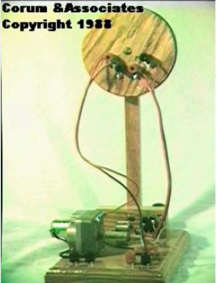
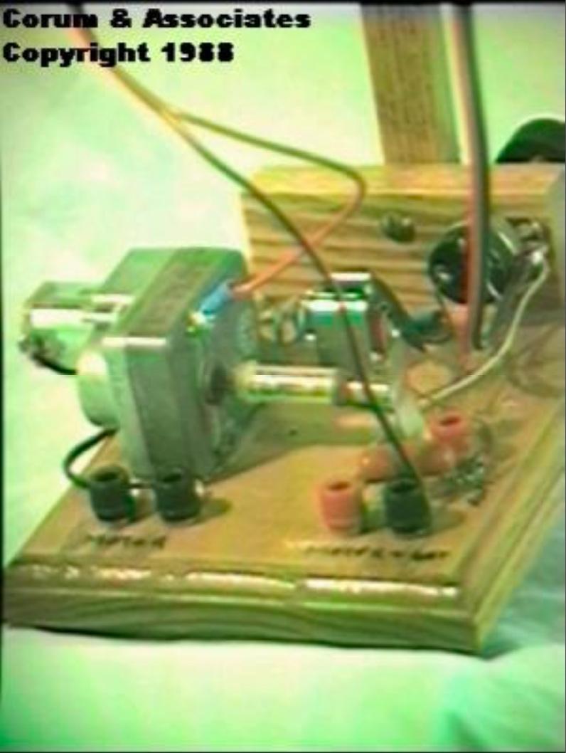
Following Tesla's circuits, we constructed several receiver models, more-or-less to the layout and specifications given his Notebook. Photos of a receiver constructed to embody the schematic of Figure 3 is shown in Figures 5 and 6. (Click on the photos to hear audio clips.) The measured parameters for the reconstructed receiver shown in the photos were as follows:

Cp = 0.1 μF (Tesla used 1/2 μF)
Cs = 500 pF
Lp = 500 μH
L_s = 100 mH
R_p = 1 Ω
R_s = 60 Ω
Q_p = 72.3
Q_s = 235
M = 450 μH
k = 0.0201
k_c = 0.0077
f_p = 22.5 kHz
f_s = 22.5 kHz
E_{coh =} 1 MΩ (open) and 50 Ω (closed)
L = RFC
r = 100 kΩ
B₁ = 9 Volts
B = 1.5 volts.

Many coherers were constructed (following Tesla's laboratory notes) and experimented with. (See CSN pg. 97 and the patents referenced in section 3.4 above.) Instead of mechanical clockworks, a small electrical motor was used to slowly rotate the coherer. Our "break" device ("d") was a TTL driven micro-relay running at 72 BPS (the same rate as Tesla's clockwork-driven break, see CSN pg. 110) with contact durations on the order of a millisecond, or so.***** Tesla reports placing the portable receivers in two boxes 9"×10"×14". His "synchronized coils" were wound on a form 10" diameter by 48" high and 24" diameter by 18" high supported on a photographic tripod (CSN, pp. 187-188). In themodel shown in Figure 5, we used interchangeable high Q pancake coils as resonators, which seemed to work satisfactorily and permitted operation on several bands.

§3.7 Analysis of the Local RF Oscillator

A circuit analysis of the coupled coils gives a "double humped" spectrum, with spectral peaks at 22.3 kHz and 22.7kHz (as would be expected with such tight coupling). The voltage across the secondary capacitor, V_cs(t), is especially interesting. It is a double side-band signal with an effective "carrier" at about 22.5 kHz (Tesla's Colorado Springs receivers operated closer to 10 kHz) and a "beat" period of 2500 μs, which corresponds to a frequency of 400 "beats per second". Interestingly, the envelope of V_c2(t) was maximum at about t = 900 μs, and the 400 hertz beats could be heard as audio pulses through the earphones.

§3.8 VLF Receiver Performance

Tesla took Branly's existing coherer element (with sensitivities on the order of 10 volts) and placed them at the high impedance end (the top) of his tuned resonators, which had voltage magnifications proportional to Q, and in so doing he increased the voltage sensitivity of the detector by a factor on the order of 200 (i.e., 46 dB). (It also gave the detector selectivity, which was something new.) He injected a local oscillator RF voltage across the coherer (by tightly link coupling the local oscillator to the resonator) for the purpose of bringing the coherer's operating point near avalanche, to further increase the sensitivity another 26 dB. Tesla discovered a technique by which the nonlinear resistance of a coherer (as a function of injected locally generated RF) could be triggered and exploited by an exterior pulse signal. The Tesla regenerative detector circuit appears to simultaneously oscillate, heterodyne, amplify, provide selectivity, and detect. Having a weak signal initiate the process and using the resulting (voltage controlled) resistance decrease to regeneratively "ratchet up" the Local Oscillator RF, which further decreased the coherer resistance, gave Tesla an improvement on the order of 70 dB in sensitivity over contemporary receiver technology. The resulting receiver tangential sensitivity was on the order of 50-500μV. And, an audio "beep" is heard each time the receiver is pulsed by an RF transient signal in the passband of its grounded spiral or helical resonator stage: the baseband earphone response is a triggered tone at the coupled oscillator beat frequency. Thisresponseisnotheardwithaconventional envelope detector. Where Tesla's receivers give "beeps", all you would hear with a communications receiver would be clicks and static.

§4 Summary

There are four modes of operation for coherer receivers:

1. Branly's mode - in which the coherer DC resistance collapses from a megohm to a few ohms when an RF signal exceeds the knee in the i-v characteristic.
2. Lodge's mode - for which the coherer crudely behaves as an analog envelope detector.
3. Bose's mode - which built on Lodge's mode,²² utilized torsional compression,²³ and was a forerunner of the point-contact diode.
4. Tesla's mode - in which locally generated RF injection exploits the voltage-controlled operating- point resistance of the coherer.

The first three modes are "passive" in that only the message signal is applied to the coherer. In modes 1 and 4 coherer agitation is required to decohere the device between pulses, and the detector does not respond well for CW. (It stays on!) Mode 2, instead of mechanical decohering, requires extreme mechanical stability. Sharp chips work best for the envelope detector mode of Lodge (which simulates crystal sets). Fine particles work best to get the go/no-go, steep-knee'd RF detector curves of Branly. But, either a strong signal is required to get operation at the knee of the characteristic curve (as Branly did), or a large bias is needed to get operation out at the knee. (The resistance is asymmetric at the knee of the characteristic curve, huge for a sinusoidal signal's negative half wave and small for its positive half wave.)

In addition to the message signal, Tesla injected a locally generated RF bias to swing the operating point, and his discovery of a controlled, frequency-selective, incremental negative resistance gave his detectors remarkable gain. Even by today's standards, his receivers were more than adequate to detect the presence of RF pulses in the 50-500 μV range. It would appear that the actual limitation on his observations was set by the ambient atmospheric noise field. It was not until Armstrong's monumental discovery of regeneration (US Patent #1,113,149) that receivers could again be made this sensitive.

APPENDIX - Negative Resistance Q-Multiplication

Consider the classical parallel tank circuit composed of passive elements, as shown in Figure 7(a). The Q of this network is given by

Q_o = $! {R_{sh} \over ω_{o}L} $!      (1)

where R = R_sh is the terminal point shunt resistance of the network measured at resonance. (For a lossless network, R_sh → ∞.) The transient response voltage of the tank is of the form

e(t) = $! {Ke {- {ω_{o} \over 2Q_{o}}t \cos \left({ω_{o} \sqrt{1 - \left({1 \over 2Q_{o}}\right)^{2}}}t\right)}} $!      (2)

which is an exponentially damped oscillation.

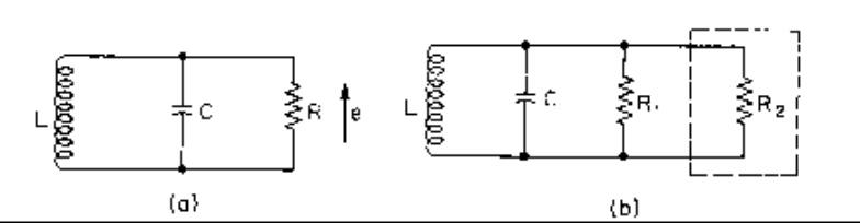
In conventional regenerative oscillators with passive tank circuits, link-coupled positive feedback is used to supply energy to overcome circuit losses. With 2-terminal negative resistance devices, such as tunnel diodes operating in the negative resistance region, negative resistance R₂ = - R_n , is injected into the passive network. The equivalent parallel load resistance is²⁴

R_eq = $! {{- R_{n} R_{sh}} \over {R_{sh} - R_{n}}} $! = $! {{R_{sh} R_{n}} \over {R_{n} - R_{sh}}} $!      (3)

which is greater than R_sh. From Equation (1), the effective Q then becomes Q_o increased by a multiplicative factor - the Q multiplier:

Q_eff = $! {R_{n} \over {R_{n} - R_{sh}}} $! Q_o      (4)

The resulting Q can be made arbitrarily large, even permitting sustained oscillations, by letting |R_n| → R_sh. This narrows the selectivity curve and magnifies the circulating current, producing substantial gain from a simple circuit with surprisingly few components.

 

* This note was condensed from material published in References 2 and 3, which may be obtained through Jim Hardesty's PV Scientific website at http://www.arcsandsparks.com.

** This is consistent with Tesla's measurement described on July 23, 1899, "... unexcited they measured more than 1,000,000 ohms while the resistance would sink down to 300 or even 50 ohms or still less when excited." Similar measured values are presented on July 28,1899.

*** The importance of this cannot be stressed strongly enough.

**** There is a surprising amount of discussion on the construction, physics, and operation of coherers in Tesla's US Patents #613,809 (Filed: July 1, 1898; Issued: Nov. 8, 1898), #685,954 (Filed: Aug. 1, 1899; Issued: Nov. 5, 1901); #685,956 (Filed: Nov. 2, 1899; Issued: Nov. 5, 1901).

***** In the Diary, July 29, 1899 (pg. 110), Tesla gives the speed of rotation of the coherers as "about 24 per minute" and the break speed as "72 per second". He also tells us that the coherer resistance was "over 1,000,000 ohms, but when excited the resistance fell almost exactly to 50 ohms."

 

References

1. Tesla, N., Nikola Tesla, Colorado Springs Notes: 1899-1900, compiled and edited by A.Marincic, Nolit, Beograd, Yugoslavia, 1978.

2. Corum, K.L., J.F. Corum, and A.H. Aidinejad, "Atmospheric Fields, Tesla's Receivers and Regenerative Detectors," Proceedings of the 1994 International Tesla Symposium, International Tesla Society, Colorado Springs, Colorado, 1994. This paper, and others, are available through PV Scientific, http://www.arcsandsparks.com.

3. Corum, K.L. and J.F. Corum, "Nikola Tesla and the Electrical Signals of Planetary Origin," presented at the 1996 International Tesla Symposium, Colorado Springs, Colorado, and at the Fifth International Tesla Conference: "Tesla III Millennium", Serbian Academy of Sciences and Arts, October 15-19, 1996, Belgrade, Yugoslavia. (The complete eighty-one page report is available through PV Scientific, http://www.arcsandsparks.com . An abbreviated synopsis, including audio clips of the receiver output, can be examined at http://teslasociety.com.)

4. Tesla, N., Nikola Tesla On His Work With Alternating Currents and Their Application to Wireless Telegraphy, Telephony, and Transmission of Power, edited by L.I. Anderson, Sun Publishing, Denver, 1992, pp. 25, 159-163.

5. Hartley, R.V.L., "Oscillations with Non-Linear Reactances," Bell System Technical Journal, Vol. 15, No. 3, July, 1936, pp. 424-440.

6. Bennett, W.R., "A General Review of Linear Varying Parameter and Nonlinear Circuit Analysis," Proc. IRE, Vol. 38, 1950, pp. 259-263.

7. Rowe, H.E., "Some General Properties of Nonlinear Elements: II. Small Signal Theory," Proc. IRE, Vol. 46, 1958, pp. 850-860.

8. Armstrong, E.H., "A Study of Heterodyne Amplificationby the Electron Relay," Proc. of IRE, Vol. 5, 1917, pp. 146- 168.

9. Armstrong, E.H., (Regenerative Feedback Invention), US Patent #1,113,149. Filed: October 29, 1913; Issued: 1914.

10. Lauer, H., and H. Brown, Radio Engineering Principles, McGraw-Hill, 1928, pg. 225.

11. Espenscheid, L. et. al., "History of some Radio Foundations," Proc. IRE, Vol. 47, 1959, pp. 1253-1268.

12. Villard, O.G. and W.L. Rorden, "Flexible Selectivity for Communications Receivers," Electronics, April, 1952, pp. 138-140.

13. McCoy, L.G., "The Heathkit Q Multiplier," QST, April, 1956, p. 39.

14. Ort, C., "Discussion," Proc. IRE, Vol. 5, 1917, pp. 163- 166.

15. Armstrong, E.H., (Superheterodyne Receiver), US Patent #1,342,885. Filed: February 8, 1919; Issued: June 8,1920.

16. Armstrong, E.H., (Superregenerative Receiver), US Patent # 1,424,065; Issued 1922.

17. Armstrong, E.H., "Some Recent Developments of Regenerative Circuits," Proc. IRE, Vol. 10, 1922, pp. 244-260.

18. Hogan, J.L., and L. Lee, Proceedings of the IRE, Vol. 1, July, 1913; and US Patent 1,141,717.

19. Ort, C., "Discussion," Proc. IRE, Vol. 5, 1917, pp. 163- 166.

20. Phillips, V.J., "The 'Italian Navy Coherer' Affair: A Turn- of-the-Century Scandal," Proc. IEE, Series A, Vol. 140, May, 1993, pp. 175-185; Reprinted in Proc. IEEE, Vol. 86, 1998, pp. 248-258.

21. Bondyopadhyay, P.K., "Sir J.C. Bose's Diode Detector Received Marconi's First Transatlantic Wireless Signal of December 1901 (The 'Italian Navy Coherer' Scandal Revisited)," Proc. IEEE, Vol. 86, 1998, pp. 259-285.

22. Sengupta, D., T.K. Sarkar, and D. Sen, "Centennial of the Semiconductor Diode Detector," Proc. IEEE, Vol. 86, 1998, pp. 235-243.

23. Bose, J.C., "Detector for Electrical Disturbances," US Patent #755,840. Filed: Sept. 30, 1901; Issued March 24, 1904. See Proc. IEEE, Vol. 86, 1998, pp. 230-234.

24. Harris, H.E., "Simplified Q Multiplier," Electronics, May, 1951, pp. 130-134.